DG Method From Scratch (in Python) - The Finite Element
and how to pick the right one for your simulation
last update: Feb 3, 2025
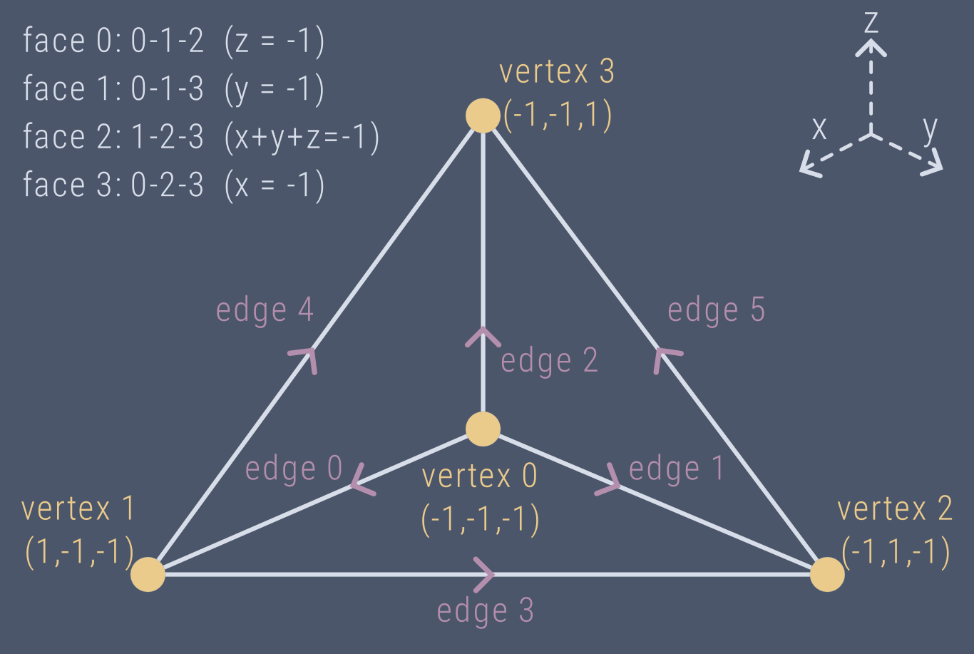
Figure 1: Geometry of a reference tetrahedron for a 3D Lagrange element.
Article Motivation
- What is a finite element?
- How does it relate to a mesh?
- Which is the right element for my simulation?
- Code it in python.
What is a finite element?
Note: were talking about specific elements that are used in finite element analysis (FEA), not the finite element method (FEM) as a whole.
A finite element is a mathematical tool that serves as building block for a numerical simulation that uses the finite element method for its spatial discretization.
The rigous mathematical definition is usually taken from The Mathematical Theory of Finite Element Methods by Brenner and Scott [1]. Their definition expands on the classic 1978 definition from P. Ciarlet [2].
A finite element is a set that contains the following three objects:
- A domain, \(\mathcal{T}\), (a subset of \(\mathbb{R}^n\) with a piecewise smooth boundary.
- A space of basis functions, \(\mathcal{V}\).
- A set of degrees of freedom, \(\mathcal{N} = {N_1, N_2, ..., N_k}\).
If you are interested in their mathematical properties, you should note that the degrees of freedom, \(\mathcal{N}\) form a basis for the dual space of P (called \(\mathcal{P'}\)).
What is the dual space of a vector space?
If \(V\) is a vector space over the real numbers \(\mathbb{R}\), then the dual space of V, denoted \(V'\) is the set of all linear functionals that map \(V \rightarrow \mathbb{R}\). This means all functions that can map a vector in \(V\) to a scalar in \(\mathbb{R}\). This includes things like summing all the elements, or finding the mean, or projecting the vector onto an axis.
If you found the set of degrees of freedom in the definition of a finite element to be confusing, its because this definition is attempting to be as general as possible, and encompass all possible types of finite elements.
Consider a very simple finite element, a Lagrange element on a tetrahedral mesh. The volume of the element is the reference tetrahedron (see fig. 1). The space of basis functions is a set of polynomials. The degrees of freedom are just the evaluation of these basis functions at specific points. In this case we can think of the nodal variables as just a set of points on the tetrahedron.
However, other elements are not so simple. Take the Nédélec element for example, which also works on a tetrahedral mesh. The volume is also a tetrahedron. The space of basis functions is also a finite polynomial space. But the Nédélec element is a H(curl)-conforming element, which means that it ensures the continuity of tangential components of the solution (necessary for electromagnetics simulations for example). To achieve this, the degrees of freedom of the lowest order 3D Nédélec element (of the first kind) are integrals over the edges of the element, of the solution doted with the tangent vector [3]
What types of finite elements exist?
A lot.
Check out DefElement for a alphabetical list of most of them.
How do I find out which element I need?
There are some questions you can ask to narrow it down:
What function space do you need?
Maxwell's equations, for example, require a curl conforming element (the curl of the field has to be continuous). Nédélec elements would be a great first choice.
What type of mesh are you using?
A tetrahedral mesh requires tetrahedral elements. Lagrange elements are a perfect first choice for tetrahedral elements with scalar unknowns.
Do you need to reduce computational time?
If you're using a parallelepiped mesh, serendipity elements might be a good starting choice.
In my case, I want to simulate ultrasound waves passing through the brain. That's a complex geometry so I want a unstructured tetrahedron mesh. I'm using a linear acoustic wave equation so Lagrange elements will be perfect to start. I can always adapt in the future. Based on this PhD thesis[4] I should start with 3rd order basis functions as they seem to scale the best.
Whats a 3rd order Lagrange element?
A third order, 3D Lagrange element is defined by the following triplet:
- A tetrahedron domain.
- A set of polynomial basis functions up to order 3.
- A set of points where the basis functions are evaluated.
Just to recap (for the sake of rigorous mathematics) the degrees of freedom of this Lagrange element are a set of points where the basis functions are evaluated. These are our unknowns that we will solve for. We can use these to recreate the solution in each cell.
That means that we have a choice of where to evaluate our basis functions. We can chose whatever quadrature points we want.
3rd order Lagrange element degrees of freedom
A common way of finding the degrees of freedom on a 3rd order Lagrange element is to choose equidistant points. Unfortunately, this can often cause unwanted oscillations in the solution due to Runge's phenomenon.
Another common choice is to make our basis functions Lagrange functions, and to evaluate them at Gauss-LobattoLegendre (GLL) points. These points are clustered towards the ends of the element, and reduce the spurious oscillations.
An even better way is to use the Warp and Blend points from Hesthaven and Warburton's book [5]. They've found a way to further reduce the oscillations by algorithmically defining the position of each point.
Theoretically, the best way would be to minimized something called the Lebesgue constant directly. The Lebesgue constant is a measure of the unwanted spurious oscillations that occur as a result of the choice of points. Francesca Rapetti et al did this for polynomial degrees up to 18 in two dimensions in their 2012 paper (see [6])
For three dimensions the best quadrature points I have seen were created by Tobin Isaac (see [7]). You can check out the implementation in the link in the references at the bottom of the page. I won't get into it here, but going forward I'll use Isaac's recursive_nodes package to find the nodal positions.
Tabulating the nodal positions
Isaac's recursive_nodes package helps us get the current state of the art coordinates for the quadrature points. It works as follows.
d = 3  # three dimensions (tetrahedra)
n = 3  # 3rd order basis functions
recursive_nodes(d,n, domain='unit')
>> [[0.         0.         0.        ]
    [0.         0.         0.2763932 ]
    [0.         0.         0.7236068 ]
    [0.         0.         1.        ]
    [0.         0.2763932  0.        ]
    [0.         0.33333333 0.33333333]
    [0.         0.2763932  0.7236068 ]
    [0.         0.7236068  0.        ]
    [0.         0.7236068  0.2763932 ]
    [0.         1.         0.        ]
    [0.2763932  0.         0.        ]
    [0.33333333 0.         0.33333333]
    [0.2763932  0.         0.7236068 ]
    [0.33333333 0.33333333 0.        ]
    [0.33333333 0.33333333 0.33333333]
    [0.2763932  0.7236068  0.        ]
    [0.7236068  0.         0.        ]
    [0.7236068  0.         0.2763932 ]
    [0.7236068  0.2763932  0.        ]
    [1.         0.         0.        ]]
Here we get the coordinates of all 20 points on a 3rd order Lagrange element on a tetrahedra.
This is wonderful, but I really only need to tabulate these points for different degrees. I don't need the whole python package. The following code can tabulate the points for up to 30th order Lagrange polynomials on a tetrahedra
import numpy as np
from recursivenodes import recursive_nodes

nodes_dict = {}
for n in range(1, 31):
    nodes_dict[str(n)] = recursive_nodes(3, n, domain='unit')  # Convert n to str for npz keys

np.savez_compressed("tetrahedra_nodes.npz", **nodes_dict)
This creates the tetrahedra_nodes.npz file that I can quickly load when defining my finite element. I can do a similar thing for the triangle nodes.
Creating the basis functions
We have our reference tetrahedron and set of nodal points with good interpolation properties. Now we need to define basis functions on the reference tetrahedron.
These need to be orthonormal basis functions on the reference tetrahedron, or else our scheme will be numerically unstable (specifically the Vandermonde matrix will be unstable).
As explained in chapter 10 of Hesthaven and Warburton's book (see [5]) if we start with a standard polynomial basis and we orthonormalize it using the Gram Schmidt method. This gives us a set of polynomials we can evaluate at any point. The Gram Schmidt process produces a lengthy polynomial, so we'll simplify it by introducing points \((a,b,c)\) that are functions of \((r,s,t)\) the nodal points on our reference tetrahedron. We'll also need to normalize the eval_jacobi function from scipy, since scipy can't do this for us.
import numpy as np
from scipy.special import eval_jacobi, gamma

def normalized_jacobi(x, n, alpha, beta):
    """
    Compute the normalized Jacobi polynomial of degree n at points x.
    """
    # Compute the unnormalized Jacobi polynomial using scipy
    P_n = eval_jacobi(n, alpha, beta, x)

    # Compute the normalization constant gamma_n
    numerator = 2 ** (alpha + beta + 1) * gamma(n + alpha + 1) * gamma(n + beta + 1)
    denominator = (2 * n + alpha + beta + 1) * gamma(n + alpha + beta + 1) * gamma(n + 1)
    gamma_n = numerator / denominator

    # Normalize the polynomial
    P_n_normalized = P_n / np.sqrt(gamma_n)

    return P_n_normalized

def orthonormal_polynomial3d(a, b, c, i, j, k):
    h1 = normalized_jacobi_p(a, 0, 0, i)
    h2 = normalized_jacobi_p(b, 2*i+1, 0, j)
    h3 = normalized_jacobi_p(c, 2*(i+j)+2, 0, k)

    P = 2 * np.sqrt(2) * h1 * h2 * ((1 - b) ** i) * h3 * ((1 - c) ** (i + j))
    return P

def rst_to_abc(r, s, t):
    """ transfer from (r,s,t) coordinates to (a,b,c) which are used to evaluate the
    jacobi polynomials in our orthonormal basis """
    Np = len(r)
    a = np.zeros(Np)
    b = np.zeros(Np)
    c = np.zeros(Np)

    for n in range(Np):
        if s[n] + t[n] != 0:
            a[n] = 2 * (1 + r[n]) / (-s[n] - t[n]) - 1
        else:
            a[n] = -1

        if t[n] != 1:
            b[n] = 2 * (1 + s[n]) / (1 - t[n]) - 1
        else:
            b[n] = -1

        c[n] = t[n]

    return a, b, c
Python Code
Lets build a python class callsed LagrangeElement for a 3rd order Lagrange element on a tetrahedron.
As we said before, this class should contain a set of points (often called the degrees of freedom) some basis functions (in this case, 3rd order Lagrange basis functions), an it should be expressed on some volume.
Do I have to make a separate element for each cell in my mesh?
No. Typically all the calculations are done on a reference element, and then mapped to each cell in the mesh via a linear affine transformation. Right now we are just going to build that reference element.
Volume: The reference tetrahedron for an unstructured mesh, with vertices at \((0,0,0), (0,1,0), (0,0,1), (1,0,0)\).
Nodal basis: We're using the optimized points from the recursivenodes code that we tabulated.
Basis functions: third order Lagrange functions. We'll use scipy's implementation of the Jacobi polynomials.
Lets start by creating a reference volume as a python class. We can then import this and use it in our LagrageElement class
import numpy as np

class Line:
    def __init__(self):
        # Define the vertices of the standard line segment
        self.vertices = np.array([0,1])

class Triangle:
    def __init__(self):
        # Define the vertices of the triangle
        self.vertices = np.array([[0, 0],
                                  [1, 0],
                                  [0, 1]])

class Tetrahedron:
    def __init__(self):
        # Define the vertices of the Tetrahedron
        self.vertices = np.array([[0, 0, 0],
                                  [1, 0, 0],
                                  [0, 1, 0],
                                  [0, 0, 1]])
import numpy as np
from reference_domains import Tetrahedron, Triangle


class LagrangeElement:
    """Lagrange finite element defined on a triangle and
      tetrahedron"""

    # load the nodes once as a class attribute
    _line_nodes = np.load("line_nodes.npz")
    _triangle_nodes = np.load("triangle_nodes.npz")
    _tetrahedron_nodes = np.load("tetrahedron_nodes.npz")

    def __init__(self, d, n):
        self.d = d  # dimension
        self.n = n  # polynomial order

        # Initialize the domain
        if d == 1:
            self.domain = Line()
        if d == 2:
            self.domain = Triangle()
        elif d == 3:
            self.domain = Tetrahedron()
        else:
            raise Exception("Incorrect element dimension (d). Should be 1, 2, or 3")

        # Load precomputed nodes
        if d == 1 and n < 31:
            self.nodes = self._line_nodes[str(n)]
        if d == 2 and n < 31:
            self.nodes = self._triangle_nodes[str(n)]
        if d == 3 and n < 31:
            self.nodes = self._tetrahedron_nodes[str(n)]
        else:
            raise Exception(f"No precomputed nodes found n={n} is not between 1 and 30")
Great, now we've got a very simple finite element. Lets plot it to see what it looks like.
Plotting
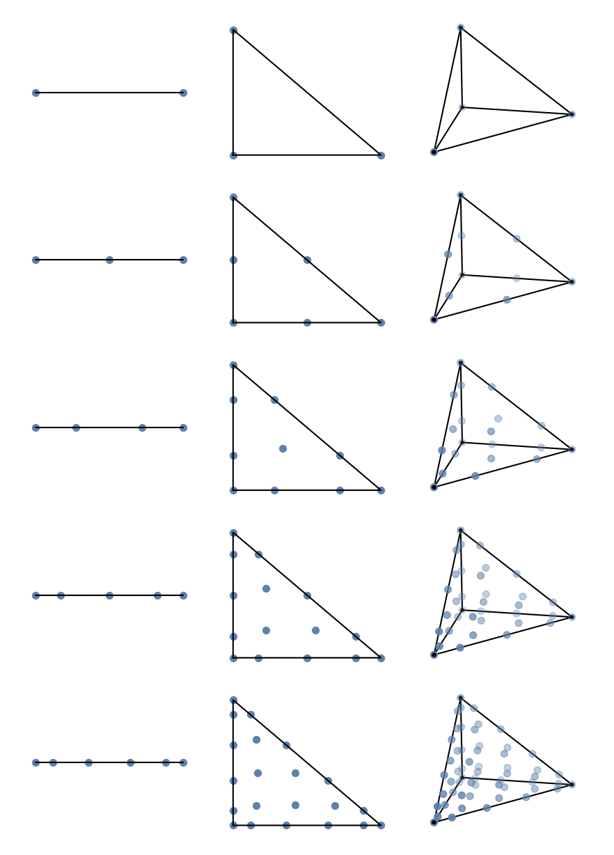
Figure 2: Grid of Lagrange Elements for various degrees of freedom (y-axis) and polynomial order (x-axis). Code is available in the plotting directory of the corresponding code in the github repo
Conclusion
We've create a python class for a Lagrange element that uses the optimal known nodal points.